Predict Rating for Yelp reviews using Naive Bayes, KNN and Logistic Regression algorithms.
The growth of the World Wide Web has resulted in troves of reviews for products we wish to purchase, destinations we may want to travel to, and decisions we make on a day to day basis. Using machine learning techniques to infer the polarity of text-based comments is of great importance in this age of information. While there have been many successful attempts at binary sentiment analysis of text-based content, fewer attempts have been made to classify texts into more granular sentiment classes. The aim of this project is to predict the star rating of
a user’s comment about a restaurant on a scale of 1, 2, 3 …to 5. Though a user self-classifies a comment on a scale of 1 to 5 in our dataset from Yelp, this research can potentially be applied to settings where a comment about a restaurant is available, but no corresponding star rating is (i.e. the sentiment expressed in review about a restaurant).
The obtained data-set is in the JSON format containing 6 million records. Some of the key statistics of Yelp dataset are as follows:
Businesses - 156,639Check-ins - 135,148Users - 1,183,362Tip - 1,028,802Reviews - 4,736,897
Yelp consists of several categories of businesses like Restaurants, Hotels, Home Service etc., of which restaurants contributed to more than 60%. As the part of the initial analysis, we considered Restaurant business and analyzed reviews of this business across multiple cities. We only used businesses and reviews data from the dataset.
{// string, 22 character unique string business id"business_id": "tnhfDv5Il8EaGSXZGiuQGg",// string, the business's name"name": "Garaje",// string, the neighborhood's name"neighborhood": "SoMa",// string, the full address of the business"address": "475 3rd St",// string, the city"city": "San Francisco",// string, 2 character state code, if applicable"state": "CA",// string, the postal code"postal code": "94107",// float, latitude"latitude": 37.7817529521,// float, longitude"longitude": -122.39612197,// float, star rating, rounded to half-stars"stars": 4.5,// interger, number of reviews"review_count": 1198,// integer, 0 or 1 for closed or open, respectively"is_open": 1,// object, business attributes to values. note: some attribute values might be objects"attributes": {"RestaurantsTakeOut": true,"BusinessParking": {"garage": false,"street": true,"validated": false,"lot": false,"valet": false},},// an array of strings of business categories"categories": ["Mexican","Burgers","Gastropubs"],// an object of key day to value hours, hours are using a 24hr clock"hours": {"Monday": "10:00-21:00","Tuesday": "10:00-21:00","Friday": "10:00-21:00","Wednesday": "10:00-21:00","Thursday": "10:00-21:00","Sunday": "11:00-18:00","Saturday": "10:00-21:00"}}
{// string, 22 character unique review id"review_id": "zdSx_SD6obEhz9VrW9uAWA",// string, 22 character unique user id, maps to the user in user.json"user_id": "Ha3iJu77CxlrFm-vQRs_8g",// string, 22 character business id, maps to business in business.json"business_id": "tnhfDv5Il8EaGSXZGiuQGg",// integer, star rating"stars": 4,// string, date formatted YYYY-MM-DD"date": "2016-03-09",// string, the review itself"text": "Great place to hang out after work: the prices are decent, and the ambience is fun. It's a bit loud, but very lively. The staff is friendly, and the food is good. They have a good selection of drinks.",// integer, number of useful votes received"useful": 0,// integer, number of funny votes received"funny": 0,// integer, number of cool votes received"cool": 0}
Firstly, the data set was in JSON format, we used some python code to convert it to CSV files. We used only business_id, categories and city from the business object and review_id, business_id, text and stars from the review object. Then we used pandas library to perform analysis and operations on CSV file. We first joined the businesses data and the reviews data and filtered out the reviews for category restaurants.
Total review count for restaurant category came out to be 2,927,731. Then we performed analysis on city wise review count. The top five cities based on review count is as follows:
Las Vegas - 849,883Phoenix - 302,403Toronto - 276,887Scottsdale - 164,893Charlotte - 141,281
We divided the data based on cities in order to perform algorithms on whole data set and part of the dataset. From the business and review combined data, we selected only review text and start rating as our main goal is to analyze text and predict the review. We created CSV files for individual cities to perform further processing.
As the part of next step - dataset preprocessing, actions taken were
We observed that in the actual dataset there were reviews businesses in Mexico. Some of them were in languages other than English. So we had to remove such reviews. For this, we used google’s langdetect library. But later when we split the data based on the cities there weren’t any reviews in foreign languages. So in the actual project, we didn’t need to do this.
Plain English text consists of a lot of stop words like the, a, as, of etc., which have very less significance in the review. We had to remove those words from the review text. We NLKT stop words library to get the stop words and remove them from the review.
Lemmatization usually refers to doing things properly with the use of a vocabulary and morphological analysis of words, normally aiming to remove inflectional endings only and to return the base or dictionary form of a word, which is known as the lemma. For example, in English, the verb ‘to walk’ may appear as ‘walk’, ‘walked’, ‘walks’, ‘walking’. The base form, ‘walk’, that one might look up in a dictionary, is called the lemma for the word. We used lemma words for words in the review. we used Word Net Lemmatizer for this purpose.
Stemming is the process of reducing derived words to their word stem. Words like “stems”, “stemmer”, “stemming”, “stemmed” as based on “stem”. For better performance of the algorithm and avoid redundancy in the dataset, we used converted each word in a review to its steam. For this used Porter Stemmer for stemming.
On the city datasets, we removed stop words first then applied lemmatization and finally stemming. At each level, we created a separate CSV file and another file with just stopwords and stemming. We performed our algorithms each of them separately to compare the effects of those preprocessing methods on accuracy. We observed that but lemmatization on words “worst” and “bad” yielded “bad”. In our 5 class classification, we needed to restore the degree of negativity in review text to correctly classify reviews. Hence we excluded lemmatization from our final process.
One of the categories that our project could fall under is definitely the supervised
learning. The main reason for this is that a prior knowledge of the target variable is already known, that needs to be predicted at the end of the project. To train our prediction models, we used three supervised learning algorithms.
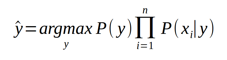
The model was build on two assumptions namely Bag of Words assumption (Assume position doesn’t matter) and Conditional Independence (Assume the feature probabilities P(xi|cj ) are independent given the class c).The model computes class probabilities for each word in feature vector for a given class (a star rating). We have used Counter class of python for calculating word frequencies which will output a dictionary with each word as key and their counts as values.
When a new feature vector(review) is given, the model calculates the probability for each class by summing all logarithmic probabilities of each word and previous class probability.
Multiplying many probabilities can result in floating-point underflow. We have used log space to reduce the underflow problem.
Then the model assigns a star rating for the given review to the class corresponding to maximum probability.
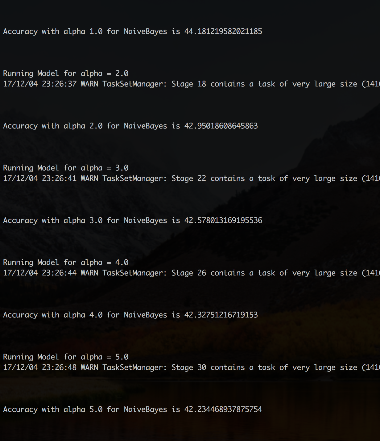
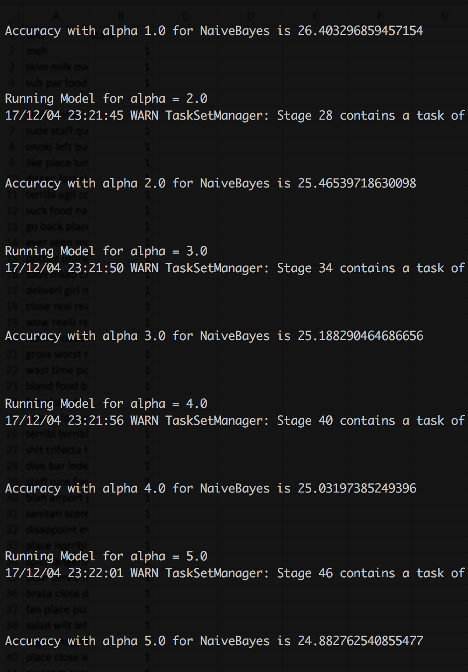
Laplace smoothing is applied to handle new words that does not exist in the training data. We have tested our model for α ranging from 1 to 5 and observed better results for α=1 and so, we have considered 1 as smoothing Laplace for our model.
K nearest neighbors is a supervised classification algorithm that uses all available data samples which classifies a new sample based on a similarity measure. There are many such similarity measures namely: Euclidean Distance, Hamming Distance, Cosine Similarity etc. Since we are working with textual data Hamming Distance best suits as the similarity measure. Hamming distance between two strings is the number of positions at which the corresponding character are different. In other words, it measures the minimum number of substitutions
required to change one string to the other or the minimum number of errors that could have transformed one string into the other.
When a new sample is to be classified, we consider a majority vote of its neighbors, with the sample being assigned to the class that is most common amongst its K nearest neighbors measured using Hamming Distance.
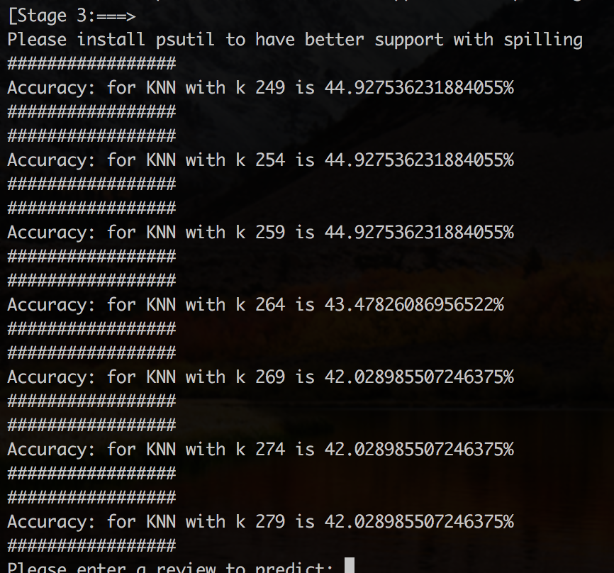
The process of choosing k value is extremely critical in the entire process. According to our research [1] we found that when k is around √N where N is number of training instances, KNN works better. So, we initialized k to √N ; ran and compared model for a delta change of 5 to initial value.
We split input review into words and chose Hamming distance measure to calculate distance between words in reviews. We tried considering TF-IDF vectors for reviews instead of just stemmed words, but TF-IDF matrix being very sparse matrix required strategical decision to be made to reduce computations.
We randomly split input dataset into training and test data in the ratio 0.009 and 0.001. Higher ratio value of test data requires very higher order cartesian products to be calculated because we were not employing feature elimination methods.
We observed that we could have implemented following feature extraction techniques and improved the performance of KNN:
Instead of considering just stemmed words of review, we could’ve considered TF-IDF values with bi-gram technique and therefore use a more contextually useful distance measure like cosine similarity.
Logistic regression is a simple classification algorithm for learning to predict a discrete variable such as predicting whether a grid of pixel intensities represents a “0” digit or a “1” digit. Here we use a hypothesis class to try to predict the probability that a given sample belongs to the class “1” versus the probability that it belongs to the class “0”. Specifically, we will try to learn a function of the form:
We performed data cleaning which include removal of punctuations, stop words and stemming (using python library function Porter Stemming) and extracted meaningful content from each review. We then constructed feature vector for each review in the dataset using python library function TfidfVectorizer imported from the package sklearn.feature_extraction.text. Inputs for TfidfVectorizer: maximum document frequency, maximum features to be extracted, language to remove stop words and ngram range.We have considered following values for inputs:
max_df=0.90 (To eliminate words with maximum frequency)max_features=500 (To retain words with highest importance and limit dimensions of the feature vectors avoiding memory out of space exception)stop_words='english'ngram_range= (1,2) (We have chosen unigrams and bigrams to capture the effect of phrases like “not good”)
Tuning Parameters: As a convergence criterion in finding beta coefficients we have fixed number of iterations to be run. For Gradient Descent to work we must set the alpha (learning rate) to an appropriate value. This parameter determines how fast or slow we will move towards the optimal coefficients. If the λ is very large we might skip the optimal solution. If it is too small, we might need too many iterations to converge to the best values. We ran our model for different alpha values and observed highest accuracy for alpha=0.001 and number of iterations=10.
To test our model, we take a review from user, add it to the training set and build tfidf vectors again using the vectorizer function mentioned above since it does not keep track of idfs of all the words.
Note: We are passing number of classes as the command line argument. We can either give it as 3-class problem or 5-class problem and the algorithm does the further computations based on the given data. After the computations of the algorithm are done it prompts user to enter a review for which it gives the computed rating.
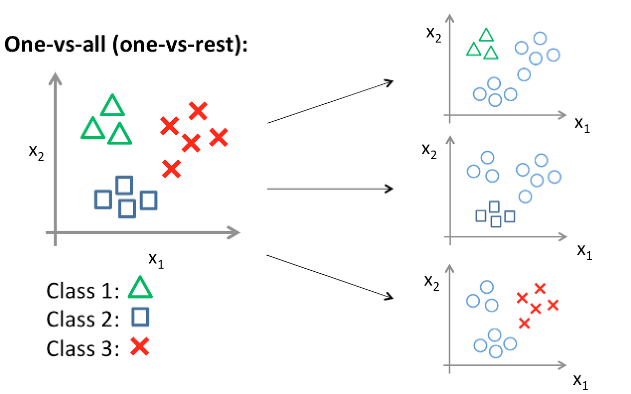
We built models for both 3-class and 5-class classification problem using above 3
supervised learning models. For 3-class classification, we programmatically constructed Good, Average and Bad classes from review labels.
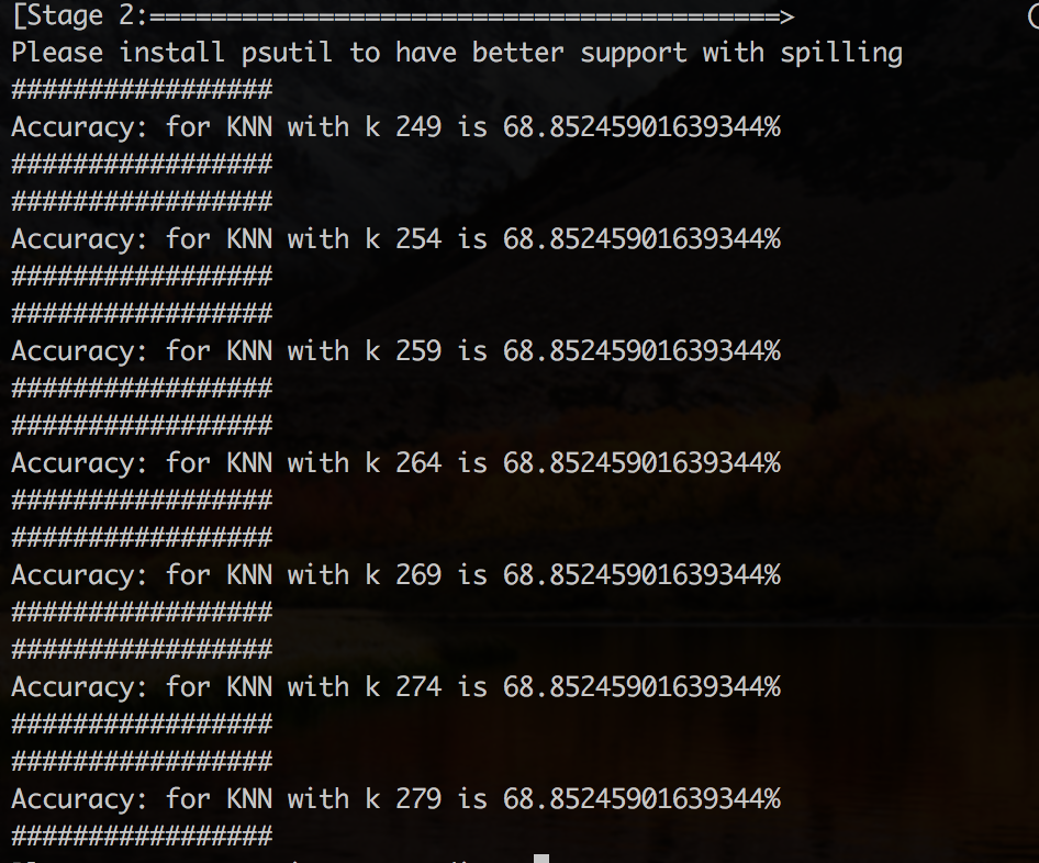
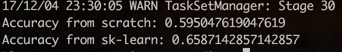
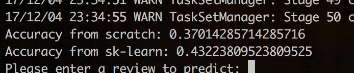
Among the three models built, Logistic Regression outperformed giving highest accuracy since TFIDFs are considered while constructing feature vectors where as in KNN we just considered the text review and hamming distance between the reviews and in Naïve Bayes we just considered word counts.
We started with 5-class problem and noticed that the words in 4-star, 5-star categories and words in 1-star, 2-star categories were very similar. So, we narrowed down our classification to a 3-class problem merging 1-star and 2-star into one class, 4-star and 5-star rating into second class and 3-star ratings as third class.
Degree of positivity or negativity was observed to be very important for 5-class classification problem. However, lemmatization of words couldn’t preserve this information (lemma of word “worst” (class-1) is “bad” (class-2)).
Because of conditional independence assumption of Naive Bayes, model failed to capture the difference between the phrases “good” and “not good”.
Built models performed better when bi-gram is chosen.