Temporal Autoencoders

This is a Keras wrapper for the simple instantiation of (deep) Autoencoder networks with
applications for dimensionality reduction of stochastic processes with respect to autocovariance.

Temporal Autoencoders can be used for timeseries dimensionality reduction.
The special thing about this application: all
linear methods (e.g. PCA and TICA) as well as commonly used nonlinear methods
(e.g. Kernel PCA) will inevitably fail on our dataset.

Linear methods will fail, since the used trajectory is generated by nonlinear embedding.
Commonly used variance based nonlinear methods such as Kernel PCA will also fail on our dataset,
since they search for “nonlinear directions” of maximal variance,
but here the variance will not yield any insight on the classification of metastable states.
We are interested in the nonlinear directions of slow processes, so to speak.

This means that we will need a nonlinear method that does not consider variance of a stationary problem,
but autocovariance at a lag time of our assumed stochastic process. In a linear setting,
this is done by τ-timelagging our data and doing component analysis
for the resulting estimated autocovariance matrix (TICA).
This idea can now be incorporated into the fitting of an autoencoder:
we will simply use timelagged observation pairs as training data of the network.

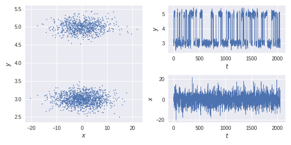
We will implement a short HMM routine to generate our test trajectory and visualize the resulting data.

Application Example

We generate a training trajectory and a test trajectory from an HMM
model with two metastable states and transform the data nonlinearly.

import numpy as np
from hmm_data import generate_trajectory
x,clusters = generate_trajectory(2000)
def transform(x):
    #transform data to a nonlinear problem
    #(x,y) -> (x,y+sqrt(abs(x)))
    y_ = x[:,1]+np.sqrt(abs(x[:,0]))
    return np.vstack([x[:,0],y_]).T
def scale(x):
    return (x-x.mean())/x.std()
traj = transform(x)
test_traj_,test_clusters = generate_trajectory(2000,start_state=1)
test_traj = transform(test_traj_)
optimal_solution = scale(test_traj_[:,1])

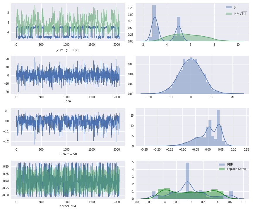
The (auto)covariance
of the transformed process in all linear subspace directions makes it impossible to detect the two states with
commonly used dimensionality reduction methods.

Application of classical methods to the HMM trajectory:

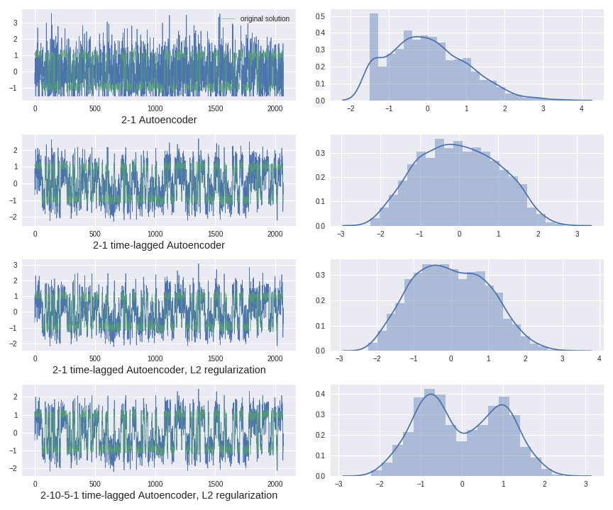
Autoencoder instantiation and training:

tau=20
autoencoder,encoder,decoder = models.Autoencoder(2,1,regularization='l2',W_penalty=0.01,b_penalty=0.01,optimizer='rmsprop')
autoencoder.fit(traj[0:-tau,:],traj[tau:,:],batch_size=32, epochs=250, verbose=0, callbacks=[], validation_split=0.0, validation_data=None, 
                shuffle=True, class_weight=None, sample_weight=None, initial_epoch=0)
encoded_traj = encoder.predict(test_traj)
encoded1 = scale(encoded_traj)

Application of different timelagged Autoencoders architectures:

References

Andreas Mardt, Luca Pasquali, Hao Wu, and Frank Noe. Vampnets: Deep learning of molecular
kinetics.Nat. Commun., 2017. in press.

L. Molgedey and H. G. Schuster. Separation of a mixture of independent signals using time
delayed correlations.Phys. Rev. Lett., 72:3634–3637, 1994.

Clarence W. Rowley, Igor Mezić, Shervin Bagheri, Philipp Schlatter, and Dan S. Henningson.
Spectral analysis of nonlinear flows.J. Fluid Mech., 641:115, nov 2009.

Peter J. Schmid. Dynamic mode decomposition of numerical and experimental data.
J. FluidMech., 656:5–28, jul 2010.

C. R. Schwantes and V. S. Pande. Modeling molecular kinetics with tica and the kernel trick.
J. Chem. Theory Comput., 11:600–608, 2015.

Jonathan H. Tu, Clarence W. Rowley, Dirk M. Luchtenburg, Steven L. Brunton, and J. Nathan
Kutz. On dynamic mode decomposition: Theory and applications.J. Comput. Dyn., 1(2):391–421, dec 2014.

M. O. Williams, I. G. Kevrekidis, and C. W. Rowley. A data–driven approximation of the
koopman operator: Extending dynamic mode decomposition.J. Nonlinear Sci., 25:1307–1346, 2015.