GNLSE: Nonlinear optics modeling tool for optical fibers

gnlse is a Python set of scripts for solving
Generalized Nonlinear Schrodringer Equation. It is one of the WUST-FOG students
projects developed by Fiber Optics Group, WUST.

Complete documentation is available at
https://gnlse.readthedocs.io.

Installation

Using pip

pip install gnlse

From scratch

1. Create a virtual environment with python -m venv gnlse or using conda.
2. Activate it with . gnlse/bin/activate.
3. Clone this repository git clone https://github.com/WUST-FOG/gnlse-python.git
4. Install gnlse package pip install . (or pip install -v -e . for develop mode) or set PYTHONPATH enviroment variable

python -m venv gnlse
. gnlse/bin/activate
git clone https://github.com/WUST-FOG/gnlse-python.git
cd gnlse-python
pip install .

Usage

We provided some examples in examples subdirectory. They can be run by typing
name of the script without any arguments.

Example:

cd gnlse-python/examples
python test_Dudley.py

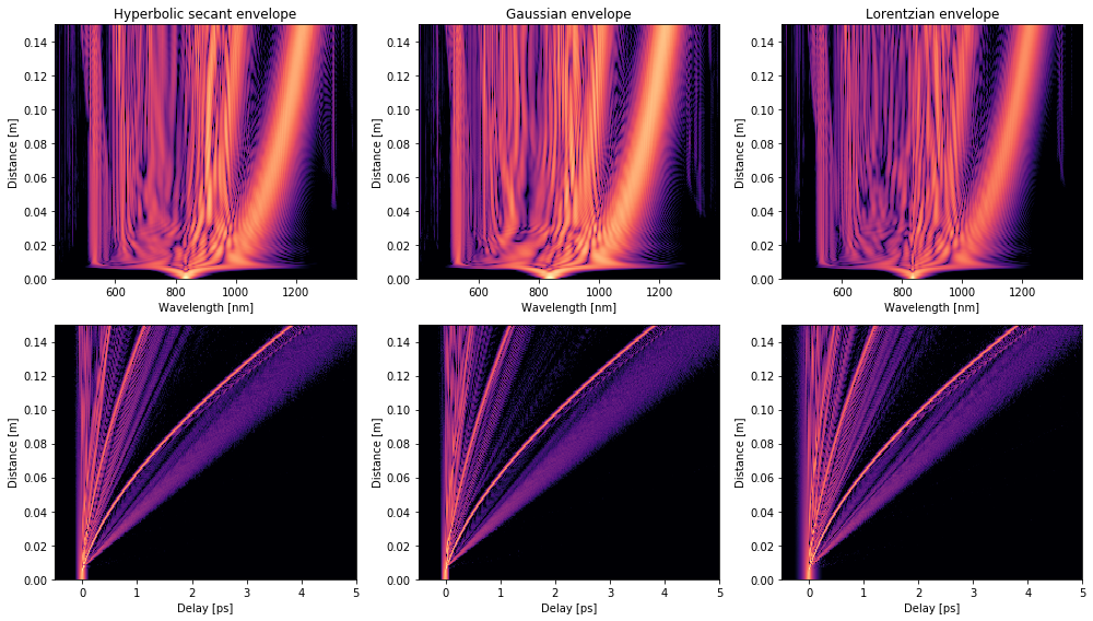
And you expect to visualise supercontinuum generation process in use of 3 types
of pulses (simulation similar to Fig.3 of Dudley et. al, RMP 78 1135 (2006)):

Major features

• Modular Design

  Main core of gnlse module is derived from the RK4IP matlab script
  written by J.C.Travers, H. Frosz and J.M. Dudley
  that is provided in “Supercontinuum Generation in Optical Fibers”,
  edited by J. M. Dudley and J. R. Taylor (Cambridge 2010).
  The toolbox prepares integration using SCIPYs ode solvers (adaptive step size).
  We decompose the solver framework into different components
  and one can easily construct a customized simulations
  by accounting different physical phenomena, ie. self stepening, Raman response.

• Raman response models

  We implement three different raman response functions:

  • ‘blowwood’: Blow and D. Wood, IEEE J. of Quant. Elec., vol. 25, no. 12, pp. 2665–2673, Dec. 1989,
  • ‘linagrawal’: Lin and Agrawal, Opt. Lett., vol. 31, no. 21, pp. 3086–3088, Nov. 2006,
  • ‘hollenbeck’: Hollenbeck and Cantrell, J. Opt. Soc. Am. B, vol. 19, no. 12, Dec. 2002.

• Nonlinearity

  We implement the possibility to account effective mode area’s dependence on frequency:

  • provide float value for gamma (effective nonlinear coefficient)
  • ‘NonlinearityFromEffectiveArea’: introduce effective mode area’s dependence on frequency (J. Laegsgaard, Opt. Express, vol. 15, no. 24, pp. 16110-16123, Nov. 2007).

• Dispersion operator

  We implement two version of dispersion operator:

  • dispersion calculated from Taylor expansion,
  • dispersion calculated from effective refractive indicies.

• Available demos

  We prepare few examples in examples subdirectory:

  • plot_input_pulse.py: plots envelope of different pulse shapes,
  • plot_Raman_response.py: plots different Raman in temporal domain,
  • test_3rd_order_soliton.py: evolution of the spectral and temporal characteristics of the 3rd order soliton,
  • test_dispersion.py: example of supercontinuum generation using different dispersion operators,
  • test_nonlinearity.py: example of supercontinuum generation using different GNLSE and M-GNLSE (take into account mode profile dispersion),
  • test_Dudley.py: example of supercontinuum generation with three types of input pulse,
  • test_gvd.py: example of pulse broadening due to group velocity dispersion,
  • test_import_export.py: example of saving file with .mat extension,
  • test_raman.py: example of soliton fision for diffrent raman response functions,
  • test_spm.py: example of self phase modulation,
  • test_spm+gvd.py: example of generation of 1st order soliton.

For more advanced examples with Coupled Generalized Nonlinear Schrodringer Equation with two modes please refer to cgnlse-python.

Release History

v2.0.1 was released in 08/01/2023.
The main branch works with python 3.9.

• 2.0.0 -> Apr 26th, 2022
  • CHANGE: Code refactor - rename envelopes module
  • FIX: Fixed extrapolation for nonlinear coefficient
• 1.1.3 -> Feb 13th, 2022
  • FIX: Shift scalling data for interpolated dispersion
• 1.1.2 -> Aug 30th, 2021
  • ADD: Continious wave envelope
  • FIX: Shift scalling data for nonlinear coefficient
• 1.1.1 -> Aug 28th, 2021
  • CHANGE: Minor bug fix with scaling
  • CHANGE: Few minor changes in the documentation
• 1.1.0 -> Aug 21st, 2021
  • Modified-GNLSE extension
  • CHANGE: Code refactor - relocate GNLSE’s attribiutes setting into constructor
  • ADD: Possibility to take into account the effective mode area’s dependence on frequency
• 1.0.0 -> Aug 13th, 2020
  • The first proper release
  • CHANGE: Complete documentation and code

Authors

• Pawel Redman
• Magda Zatorska
• Adam Pawlowski
• Daniel Szulc
• Sylwia Majchrowska
• Karol Tarnowski

Acknowledgement

gnlse-python is an open source project that is contributed by researchers,
engineers, and students from Wroclaw University of Science and Technology
as a part of Fiber Optics Group’s nonlinear simulations projects.
The python code based on MATLAB code published in
‘Supercontinuum Generation in Optical Fibers’
by J. M. Dudley and J. R. Taylor, available at
http://scgbook.info/.

Citation

If you find this code useful in your research, please consider citing:

@misc{redman2021gnlsepython,
      title={gnlse-python: Open Source Software to Simulate
             Nonlinear Light Propagation In Optical Fibers}, 
      author={Pawel Redman and Magdalena Zatorska and Adam Pawlowski
              and Daniel Szulc and Sylwia Majchrowska and Karol Tarnowski},
      year={2021},
      eprint={2110.00298},
      archivePrefix={arXiv},
      primaryClass={physics.optics}
}

Contributing

Pull requests are welcome.
For major changes, please open an issue first to discuss
what you would like to change.

Please make sure to update example tests as appropriate.

License

MIT